It is a well known fact that data scientists spend the majority of their time cleaning and wrangling data before they begin to start to model a problem. For a well defined problem with relatively clean data and knowledge of the problem domain, the time taken is far less. But when tasked with a problem that we aren’t as knowledgeable about, how can a data scientist make the best use of his time to determine whether a problem is solvable with the data provided?
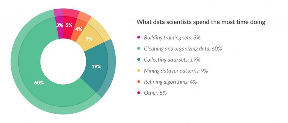
Forbes findings confirm the above statement.
Enter Rapid Prototyping
This is my personal take on determining whether a project can be completed given the data at hand.
The goal of Rapid Prototyping is simple:
What is the simplest and fastest model implementation that will give us a baseline working prototype?
The concern any data scientist will have now is that: We want to build a model but we have yet to focus on that data. And without knowledge of the problem domain, how can we determine what features we should generate and use to implement this solution? I’ll answer the question of feature selection shortly, but first let’s look at how we’ll automatically generate meaningful features.
Deep Feature Synthesis
Invented by MIT and first showcased in 2015, Deep Feature Synthesis was originally designed to speed up the process of building predictive models on multi-table datasets.
Deep feature Synthesis has three key concepts:
1. Deriving features from relationships in the data
2. Features are generated by using simple mathematics across datasets
3. New features are created from previously derived features
for more reading on this, check out the FeatureLabs blog post.
Our main reason for using Deep Feature Synthesis for Rapid Prototyping is to take away the need for the knowledge of the problem domain by fully automating the feature generation. DFS can create very complex features by stacking primitives (basic operations on the data) within a singular dataset and across relational tables.
As for how we’ll select features, we’ll use the primitives generated by DFS and remove any highly correlated features and use this as our feature set.
Rapid Prototyping with Deep Feature Synthesis by Example - The Titanic
I thought it apt as my maiden (pun intended) post to use the Titanic dataset to demonstrate the idea of rapid prototyping. The goal here is to create the simplest baseline model to prove that this problem can be solved. For those unfamiliar with the Titanic data (albeit, if you’re reading this you probably know exactly what I’m talking about), the goal is to predict whether a passenger survived given a set of features. A binary classification problem.
We start by reading in the data and taking a quick look at what’s there:
train = pd.read_csv("train.csv")
test = pd.read_csv("test.csv")
train.head()
| PassengerId | Survived | Pclass | Name | Sex | Age | SibSp | Parch | Ticket | Fare | Cabin | Embarked | |
|---|---|---|---|---|---|---|---|---|---|---|---|---|
| 0 | 1 | 0 | 3 | Braund, Mr. Owen Harris | male | 22.0 | 1 | 0 | A/5 21171 | 7.2500 | NaN | S |
| 1 | 2 | 1 | 1 | Cumings, Mrs. John Bradley (Florence Briggs Th... | female | 38.0 | 1 | 0 | PC 17599 | 71.2833 | C85 | C |
| 2 | 3 | 1 | 3 | Heikkinen, Miss. Laina | female | 26.0 | 0 | 0 | STON/O2. 3101282 | 7.9250 | NaN | S |
| 3 | 4 | 1 | 1 | Futrelle, Mrs. Jacques Heath (Lily May Peel) | female | 35.0 | 1 | 0 | 113803 | 53.1000 | C123 | S |
| 4 | 5 | 0 | 3 | Allen, Mr. William Henry | male | 35.0 | 0 | 0 | 373450 | 8.0500 | NaN | S |
Now we look at rapid prototyping, lets impute data in the most simplest way or drop it if we need to.
# Fill the age with the median value

median_age_train = train.Age.median()

# Fill missing Age, forward fill embarked, drop what we may not need for rapid prototyping
train.Age.fillna(median_age_train, inplace=True)
train.Embarked.fillna(method='ffill', inplace=True)
train.drop(['Name', 'Cabin', 'Ticket'], axis=1, inplace=True)

median_age_test = test.Age.median() # set median value

# fill NAN data
test.Age.fillna(median_age_test, inplace=True)
test.drop(['Name', 'Cabin', 'Ticket'], axis=1, inplace=True)
The second step after imputing is to automate feature engineering and to do this we use the featuretools package for deep feature synthesis. The featuretools package has two types of primitives, namely aggregation and transformation:
Aggregation
primitives = ft.list_primitives()
pd.options.display.max_colwidth = 100
primitives[primitives['type'] == 'aggregation'].head(primitives[primitives['type'] == 'aggregation'].shape[0])
| name | type | description | |
|---|---|---|---|
| 0 | num_true | aggregation | Counts the number of `True` values. |
| 1 | std | aggregation | Computes the dispersion relative to the mean value, ignoring `NaN`. |
| 2 | sum | aggregation | Calculates the total addition, ignoring `NaN`. |
| 3 | count | aggregation | Determines the total number of values, excluding `NaN`. |
| 4 | num_unique | aggregation | Determines the number of distinct values, ignoring `NaN` values. |
| 5 | skew | aggregation | Computes the extent to which a distribution differs from a normal distribution. |
| 6 | time_since_last | aggregation | Calculates the time elapsed since the last datetime (in seconds). |
| 7 | time_since_first | aggregation | Calculates the time elapsed since the first datetime (in seconds). |
| 8 | max | aggregation | Calculates the highest value, ignoring `NaN` values. |
| 9 | median | aggregation | Determines the middlemost number in a list of values. |
| 10 | avg_time_between | aggregation | Computes the average number of seconds between consecutive events. |
| 11 | all | aggregation | Calculates if all values are 'True' in a list. |
| 12 | trend | aggregation | Calculates the trend of a variable over time. |
| 13 | min | aggregation | Calculates the smallest value, ignoring `NaN` values. |
| 14 | any | aggregation | Determines if any value is 'True' in a list. |
| 15 | n_most_common | aggregation | Determines the `n` most common elements. |
| 16 | percent_true | aggregation | Determines the percent of `True` values. |
| 17 | mode | aggregation | Determines the most commonly repeated value. |
| 18 | last | aggregation | Determines the last value in a list. |
| 19 | mean | aggregation | Computes the average for a list of values. |
Transformation
primitives[primitives['type'] == 'transform'].head(primitives[primitives['type'] == 'transform'].shape[0])
| name | type | description | |
|---|---|---|---|
| 20 | haversine | transform | Calculates the approximate haversine distance between two LatLong |
| 21 | multiply_numeric_scalar | transform | Multiply each element in the list by a scalar. |
| 22 | less_than_equal_to_scalar | transform | Determines if values are less than or equal to a given scalar. |
| 23 | modulo_by_feature | transform | Return the modulo of a scalar by each element in the list. |
| 24 | num_characters | transform | Calculates the number of characters in a string. |
| 25 | time_since_previous | transform | Compute the time in seconds since the previous instance of an entry. |
| 26 | is_null | transform | Determines if a value is null. |
| 27 | or | transform | Element-wise logical OR of two lists. |
| 28 | latitude | transform | Returns the first tuple value in a list of LatLong tuples. |
| 29 | scalar_subtract_numeric_feature | transform | Subtract each value in the list from a given scalar. |
| 30 | is_weekend | transform | Determines if a date falls on a weekend. |
| 31 | less_than_scalar | transform | Determines if values are less than a given scalar. |
| 32 | modulo_numeric | transform | Element-wise modulo of two lists. |
| 33 | not | transform | Negates a boolean value. |
| 34 | subtract_numeric | transform | Element-wise subtraction of two lists. |
| 35 | divide_numeric_scalar | transform | Divide each element in the list by a scalar. |
| 36 | greater_than_equal_to_scalar | transform | Determines if values are greater than or equal to a given scalar. |
| 37 | month | transform | Determines the month value of a datetime. |
| 38 | cum_max | transform | Calculates the cumulative maximum. |
| 39 | add_numeric | transform | Element-wise addition of two lists. |
| 40 | diff | transform | Compute the difference between the value in a list and the |
| 41 | greater_than_scalar | transform | Determines if values are greater than a given scalar. |
| 42 | minute | transform | Determines the minutes value of a datetime. |
| 43 | cum_mean | transform | Calculates the cumulative mean. |
| 44 | days_since | transform | Calculates the number of days from a value to a specified datetime. |
| 45 | not_equal | transform | Determines if values in one list are not equal to another list. |
| 46 | hour | transform | Determines the hour value of a datetime. |
| 47 | cum_sum | transform | Calculates the cumulative sum. |
| 48 | divide_numeric | transform | Element-wise division of two lists. |
| 49 | and | transform | Element-wise logical AND of two lists. |
| 50 | equal | transform | Determines if values in one list are equal to another list. |
| 51 | num_words | transform | Determines the number of words in a string by counting the spaces. |
| 52 | time_since | transform | Calculates time in nanoseconds from a value to a specified cutoff datetime. |
| 53 | longitude | transform | Returns the second tuple value in a list of LatLong tuples. |
| 54 | absolute | transform | Computes the absolute value of a number. |
| 55 | less_than_equal_to | transform | Determines if values in one list are less than or equal to another list. |
| 56 | modulo_numeric_scalar | transform | Return the modulo of each element in the list by a scalar. |
| 57 | multiply_numeric | transform | Element-wise multiplication of two lists. |
| 58 | weekday | transform | Determines the day of the week from a datetime. |
| 59 | percentile | transform | Determines the percentile rank for each value in a list. |
| 60 | subtract_numeric_scalar | transform | Subtract a scalar from each element in the list. |
| 61 | divide_by_feature | transform | Divide a scalar by each value in the list. |
| 62 | less_than | transform | Determines if values in one list are less than another list. |
| 63 | year | transform | Determines the year value of a datetime. |
| 64 | add_numeric_scalar | transform | Add a scalar to each value in the list. |
| 65 | negate | transform | Negates a numeric value. |
| 66 | greater_than_equal_to | transform | Determines if values in one list are greater than or equal to another list. |
| 67 | week | transform | Determines the week of the year from a datetime. |
| 68 | cum_min | transform | Calculates the cumulative minimum. |
| 69 | isin | transform | Determines whether a value is present in a provided list. |
| 70 | not_equal_scalar | transform | Determines if values in a list are not equal to a given scalar. |
| 71 | greater_than | transform | Determines if values in one list are greater than another list. |
| 72 | second | transform | Determines the seconds value of a datetime. |
| 73 | cum_count | transform | Calculates the cumulative count. |
| 74 | equal_scalar | transform | Determines if values in a list are equal to a given scalar. |
| 75 | day | transform | Determines the day of the month from a datetime. |
The aggregation features are very simple, while the transformation features tend to be a bit more complex. Stacking these automated features on top of each other creates more complex features that may be better predictors. The idea here is that we want to abstract ourselves away from needing domain knowledge in the short term as, if the problem can be solved relatively simply, we can spend more time developing deeper, domain specific features after we’ve proved the problem can be solved.
Deep Feature Synthesis - Coded
# Create the full dataset with both training and test data
full = train.append(test)
passenger_id=test['PassengerId']
We need to do a bit of cleanup on categorical variables to apply deep feature synthesis, our initial features need to be numeric.
# replace missing Fare
full.Fare.fillna(full.Fare.mean(), inplace=True)

# Encode Gender
full['Sex'] = full.Sex.apply(lambda x: 0 if x == "female" else 1)

# Encode Embarked
full['Embarked'] = full['Embarked'].map( {'S': 0, 'C': 1, 'Q': 2} ).astype(int)

# replace all other missing with 0
full.fillna(0, inplace=True)
Next we create the entity set, this defines the DataFrame and what each variable data type is (the default is a continuous numeric)
# We create an entity set
es = ft.EntitySet(id = 'titanic')

es = es.entity_from_dataframe(entity_id = 'full', dataframe = full.drop(['Survived'], axis=1),
                              variable_types =
                              {
                                  'Embarked': ft.variable_types.Categorical,
                                  'Sex': ft.variable_types.Boolean
                              },
                              index = 'PassengerId')

es
Entityset: titanic
  Entities:
    full [Rows: 1309, Columns: 8]
  Relationships:
    No relationships
We then normalize the entries, this isn’t normalization in the traditional data science sense. This is a creation of relationships between the large dataset and lookups into the mapped features:
es = es.normalize_entity(base_entity_id='full', new_entity_id='Embarked', index='Embarked')
es = es.normalize_entity(base_entity_id='full', new_entity_id='Sex', index='Sex')
es = es.normalize_entity(base_entity_id='full', new_entity_id='Pclass', index='Pclass')
es = es.normalize_entity(base_entity_id='full', new_entity_id='Parch', index='Parch')
es = es.normalize_entity(base_entity_id='full', new_entity_id='SibSp', index='SibSp')
es
Entityset: titanic
  Entities:
    full [Rows: 1309, Columns: 8]
    Embarked [Rows: 3, Columns: 1]
    Sex [Rows: 2, Columns: 1]
    Pclass [Rows: 3, Columns: 1]
    Parch [Rows: 8, Columns: 1]
    SibSp [Rows: 7, Columns: 1]
  Relationships:
    full.Embarked -> Embarked.Embarked
    full.Sex -> Sex.Sex
    full.Pclass -> Pclass.Pclass
    full.Parch -> Parch.Parch
    full.SibSp -> SibSp.SibSp
What we’ve done here is defined entities for each of the features and related them to the DataFrame we use. These new entities contain unique values of the features within the original DataFrame. We can now run the deep feature synthesis:
features, feature_names = ft.dfs(entityset = es,
                                 target_entity = 'full',
                                 max_depth = 2)
len(feature_names)
112
Within a few seconds we’ve generated 112 features from the 5 we originally had! Some of these may not be useful and we’d want to remove any variables that are highly correlated (or collinear).
# Threshold for removing correlated variables
threshold = 0.95

# Absolute value correlation matrix
corr_matrix = features.corr().abs()
upper = corr_matrix.where(np.triu(np.ones(corr_matrix.shape), k=1).astype(np.bool))
upper.head(50)
| Age | Fare | Parch | Pclass | SibSp | Embarked | Sex | Embarked.SUM(full.Age) | Embarked.SUM(full.Fare) | Embarked.STD(full.Age) | ... | SibSp.MEAN(full.Fare) | SibSp.COUNT(full) | SibSp.NUM_UNIQUE(full.Parch) | SibSp.NUM_UNIQUE(full.Pclass) | SibSp.NUM_UNIQUE(full.Embarked) | SibSp.NUM_UNIQUE(full.Sex) | SibSp.MODE(full.Parch) | SibSp.MODE(full.Pclass) | SibSp.MODE(full.Embarked) | SibSp.MODE(full.Sex) | |
|---|---|---|---|---|---|---|---|---|---|---|---|---|---|---|---|---|---|---|---|---|---|
| Age | NaN | 0.180519 | 0.125677 | 0.380274 | 0.188920 | 0.022174 | 0.052928 | 0.040441 | 0.008514 | 0.045555 | ... | 6.079957e-02 | 1.308523e-01 | 1.976589e-01 | 2.133987e-01 | 2.012332e-01 | NaN | 2.379074e-01 | NaN | NaN | 2.282128e-02 |
| Fare | NaN | NaN | 0.221522 | 0.558477 | 0.160224 | 0.064135 | 0.185484 | 0.136867 | 0.010706 | 0.193481 | ... | 2.256391e-01 | 2.089606e-01 | 4.979847e-02 | 3.105973e-02 | 9.761043e-02 | NaN | 6.134832e-02 | NaN | NaN | 1.914642e-01 |
| Parch | NaN | NaN | NaN | 0.018322 | 0.373587 | 0.096857 | 0.213125 | 0.083092 | 0.102642 | 0.091228 | ... | 3.302803e-01 | 3.625643e-01 | 5.262633e-02 | 2.650650e-01 | 2.781161e-01 | NaN | 2.938461e-01 | NaN | NaN | 2.488658e-01 |
| Pclass | NaN | NaN | NaN | NaN | 0.060832 | 0.033373 | 0.124617 | 0.051522 | 0.091441 | 0.280068 | ... | 9.321064e-02 | 5.610448e-02 | 2.076503e-01 | 1.435907e-01 | 1.240303e-01 | NaN | 1.488672e-01 | NaN | NaN | 1.623380e-01 |
| SibSp | NaN | NaN | NaN | NaN | NaN | 0.074966 | 0.109609 | 0.076507 | 0.070912 | 0.032782 | ... | 7.100906e-01 | 8.101948e-01 | 4.109176e-01 | 7.593949e-01 | 7.792276e-01 | NaN | 8.217369e-01 | NaN | NaN | 3.515147e-01 |
| Embarked | NaN | NaN | NaN | NaN | NaN | NaN | 0.124849 | 0.966496 | 0.983744 | 0.604985 | ... | 7.474154e-02 | 5.931944e-02 | 2.727147e-02 | 3.287548e-02 | 8.961550e-02 | NaN | 5.740721e-02 | NaN | NaN | 4.370091e-02 |
| Sex | NaN | NaN | NaN | NaN | NaN | NaN | NaN | 0.123637 | 0.120740 | 0.066315 | ... | 1.925157e-01 | 1.773133e-01 | 8.506071e-02 | 1.654746e-03 | 4.743528e-02 | NaN | 2.062120e-02 | NaN | NaN | 1.868998e-01 |
| Embarked.SUM(full.Age) | NaN | NaN | NaN | NaN | NaN | NaN | NaN | NaN | 0.904692 | 0.380337 | ... | 5.080938e-02 | 4.266879e-02 | 6.158505e-02 | 5.262555e-02 | 1.046465e-01 | NaN | 7.803594e-02 | NaN | NaN | 1.143051e-02 |
| Embarked.SUM(full.Fare) | NaN | NaN | NaN | NaN | NaN | NaN | NaN | NaN | NaN | 0.738135 | ... | 8.851772e-02 | 6.861361e-02 | 2.182977e-03 | 1.775324e-02 | 7.554246e-02 | NaN | 4.069646e-02 | NaN | NaN | 6.454272e-02 |
| Embarked.STD(full.Age) | NaN | NaN | NaN | NaN | NaN | NaN | NaN | NaN | NaN | NaN | ... | 1.116884e-01 | 8.137341e-02 | 9.277791e-02 | 4.479328e-02 | 1.724522e-03 | NaN | 3.522716e-02 | NaN | NaN | 1.220009e-01 |
| Embarked.STD(full.Fare) | NaN | NaN | NaN | NaN | NaN | NaN | NaN | NaN | NaN | NaN | ... | 6.863038e-02 | 4.548945e-02 | 1.399096e-01 | 8.583273e-02 | 8.526836e-02 | NaN | 9.677419e-02 | NaN | NaN | 1.101666e-01 |
| Embarked.MAX(full.Age) | NaN | NaN | NaN | NaN | NaN | NaN | NaN | NaN | NaN | NaN | ... | 3.953760e-02 | 3.467741e-02 | 7.500714e-02 | 6.000096e-02 | 1.089434e-01 | NaN | 8.526941e-02 | NaN | NaN | 2.605402e-03 |
| Embarked.MAX(full.Fare) | NaN | NaN | NaN | NaN | NaN | NaN | NaN | NaN | NaN | NaN | ... | 7.869541e-02 | 5.334542e-02 | 1.386663e-01 | 8.311418e-02 | 7.566791e-02 | NaN | 9.124495e-02 | NaN | NaN | 1.170830e-01 |
| Embarked.SKEW(full.Age) | NaN | NaN | NaN | NaN | NaN | NaN | NaN | NaN | NaN | NaN | ... | 1.117975e-01 | 8.235227e-02 | 7.634822e-02 | 3.321729e-02 | 1.505507e-02 | NaN | 2.028997e-02 | NaN | NaN | 1.151055e-01 |
| Embarked.SKEW(full.Fare) | NaN | NaN | NaN | NaN | NaN | NaN | NaN | NaN | NaN | NaN | ... | 8.041969e-02 | 5.470374e-02 | 1.382240e-01 | 8.248716e-02 | 7.379029e-02 | NaN | 9.008990e-02 | NaN | NaN | 1.181705e-01 |
| Embarked.MIN(full.Age) | NaN | NaN | NaN | NaN | NaN | NaN | NaN | NaN | NaN | NaN | ... | 1.042943e-01 | 7.866970e-02 | 3.734317e-02 | 7.157385e-03 | 4.846077e-02 | NaN | 1.177652e-02 | NaN | NaN | 9.299433e-02 |
| Embarked.MIN(full.Fare) | NaN | NaN | NaN | NaN | NaN | NaN | NaN | NaN | NaN | NaN | ... | 6.626721e-02 | 5.348169e-02 | 4.049116e-02 | 4.062107e-02 | 9.602416e-02 | NaN | 6.568088e-02 | NaN | NaN | 3.181999e-02 |
| Embarked.MEAN(full.Age) | NaN | NaN | NaN | NaN | NaN | NaN | NaN | NaN | NaN | NaN | ... | 5.853642e-02 | 3.771210e-02 | 1.392973e-01 | 8.725143e-02 | 9.300786e-02 | NaN | 1.006344e-01 | NaN | NaN | 1.024409e-01 |
| Embarked.MEAN(full.Fare) | NaN | NaN | NaN | NaN | NaN | NaN | NaN | NaN | NaN | NaN | ... | 6.548557e-02 | 4.305673e-02 | 1.398962e-01 | 8.639949e-02 | 8.785982e-02 | NaN | 9.813762e-02 | NaN | NaN | 1.078349e-01 |
| Embarked.COUNT(full) | NaN | NaN | NaN | NaN | NaN | NaN | NaN | NaN | NaN | NaN | ... | 4.855874e-02 | 4.107968e-02 | 6.438503e-02 | 5.418260e-02 | 1.056263e-01 | NaN | 7.958898e-02 | NaN | NaN | 8.577004e-03 |
| Embarked.NUM_UNIQUE(full.Parch) | NaN | NaN | NaN | NaN | NaN | NaN | NaN | NaN | NaN | NaN | ... | 3.634142e-02 | 3.239726e-02 | 7.855319e-02 | 6.190952e-02 | 1.098979e-01 | NaN | 8.708501e-02 | NaN | NaN | 6.475036e-03 |
| Embarked.NUM_UNIQUE(full.Pclass) | NaN | NaN | NaN | NaN | NaN | NaN | NaN | NaN | NaN | NaN | ... | NaN | NaN | NaN | NaN | NaN | NaN | NaN | NaN | NaN | NaN |
| Embarked.NUM_UNIQUE(full.SibSp) | NaN | NaN | NaN | NaN | NaN | NaN | NaN | NaN | NaN | NaN | ... | 2.014379e-02 | 2.075504e-02 | 9.492864e-02 | 7.045971e-02 | 1.131144e-01 | NaN | 9.484037e-02 | NaN | NaN | 2.540821e-02 |
| Embarked.NUM_UNIQUE(full.Sex) | NaN | NaN | NaN | NaN | NaN | NaN | NaN | NaN | NaN | NaN | ... | NaN | NaN | NaN | NaN | NaN | NaN | NaN | NaN | NaN | NaN |
| Embarked.MODE(full.Parch) | NaN | NaN | NaN | NaN | NaN | NaN | NaN | NaN | NaN | NaN | ... | NaN | NaN | NaN | NaN | NaN | NaN | NaN | NaN | NaN | NaN |
| Embarked.MODE(full.Pclass) | NaN | NaN | NaN | NaN | NaN | NaN | NaN | NaN | NaN | NaN | ... | 3.844424e-02 | 2.245797e-02 | 1.339125e-01 | 8.714516e-02 | 1.041817e-01 | NaN | 1.045429e-01 | NaN | NaN | 8.529384e-02 |
| Embarked.MODE(full.SibSp) | NaN | NaN | NaN | NaN | NaN | NaN | NaN | NaN | NaN | NaN | ... | NaN | NaN | NaN | NaN | NaN | NaN | NaN | NaN | NaN | NaN |
| Embarked.MODE(full.Sex) | NaN | NaN | NaN | NaN | NaN | NaN | NaN | NaN | NaN | NaN | ... | NaN | NaN | NaN | NaN | NaN | NaN | NaN | NaN | NaN | NaN |
| Sex.SUM(full.Age) | NaN | NaN | NaN | NaN | NaN | NaN | NaN | NaN | NaN | NaN | ... | 1.925157e-01 | 1.773133e-01 | 8.506071e-02 | 1.654746e-03 | 4.743528e-02 | NaN | 2.062120e-02 | NaN | NaN | 1.868998e-01 |
| Sex.SUM(full.Fare) | NaN | NaN | NaN | NaN | NaN | NaN | NaN | NaN | NaN | NaN | ... | 1.925157e-01 | 1.773133e-01 | 8.506071e-02 | 1.654746e-03 | 4.743528e-02 | NaN | 2.062120e-02 | NaN | NaN | 1.868998e-01 |
| Sex.STD(full.Age) | NaN | NaN | NaN | NaN | NaN | NaN | NaN | NaN | NaN | NaN | ... | 1.925157e-01 | 1.773133e-01 | 8.506071e-02 | 1.654746e-03 | 4.743528e-02 | NaN | 2.062120e-02 | NaN | NaN | 1.868998e-01 |
| Sex.STD(full.Fare) | NaN | NaN | NaN | NaN | NaN | NaN | NaN | NaN | NaN | NaN | ... | 1.925157e-01 | 1.773133e-01 | 8.506071e-02 | 1.654746e-03 | 4.743528e-02 | NaN | 2.062120e-02 | NaN | NaN | 1.868998e-01 |
| Sex.MAX(full.Age) | NaN | NaN | NaN | NaN | NaN | NaN | NaN | NaN | NaN | NaN | ... | 1.925157e-01 | 1.773133e-01 | 8.506071e-02 | 1.654746e-03 | 4.743528e-02 | NaN | 2.062120e-02 | NaN | NaN | 1.868998e-01 |
| Sex.MAX(full.Fare) | NaN | NaN | NaN | NaN | NaN | NaN | NaN | NaN | NaN | NaN | ... | 3.665734e-14 | 2.195949e-16 | 3.351113e-16 | 1.484102e-15 | 2.188883e-15 | NaN | 4.885604e-16 | NaN | NaN | 2.207137e-16 |
| Sex.SKEW(full.Age) | NaN | NaN | NaN | NaN | NaN | NaN | NaN | NaN | NaN | NaN | ... | 1.925157e-01 | 1.773133e-01 | 8.506071e-02 | 1.654746e-03 | 4.743528e-02 | NaN | 2.062120e-02 | NaN | NaN | 1.868998e-01 |
| Sex.SKEW(full.Fare) | NaN | NaN | NaN | NaN | NaN | NaN | NaN | NaN | NaN | NaN | ... | 1.925157e-01 | 1.773133e-01 | 8.506071e-02 | 1.654746e-03 | 4.743528e-02 | NaN | 2.062120e-02 | NaN | NaN | 1.868998e-01 |
| Sex.MIN(full.Age) | NaN | NaN | NaN | NaN | NaN | NaN | NaN | NaN | NaN | NaN | ... | 1.925157e-01 | 1.773133e-01 | 8.506071e-02 | 1.654746e-03 | 4.743528e-02 | NaN | 2.062120e-02 | NaN | NaN | 1.868998e-01 |
| Sex.MIN(full.Fare) | NaN | NaN | NaN | NaN | NaN | NaN | NaN | NaN | NaN | NaN | ... | 1.925157e-01 | 1.773133e-01 | 8.506071e-02 | 1.654746e-03 | 4.743528e-02 | NaN | 2.062120e-02 | NaN | NaN | 1.868998e-01 |
| Sex.MEAN(full.Age) | NaN | NaN | NaN | NaN | NaN | NaN | NaN | NaN | NaN | NaN | ... | 1.925157e-01 | 1.773133e-01 | 8.506071e-02 | 1.654746e-03 | 4.743528e-02 | NaN | 2.062120e-02 | NaN | NaN | 1.868998e-01 |
| Sex.MEAN(full.Fare) | NaN | NaN | NaN | NaN | NaN | NaN | NaN | NaN | NaN | NaN | ... | 1.925157e-01 | 1.773133e-01 | 8.506071e-02 | 1.654746e-03 | 4.743528e-02 | NaN | 2.062120e-02 | NaN | NaN | 1.868998e-01 |
| Sex.COUNT(full) | NaN | NaN | NaN | NaN | NaN | NaN | NaN | NaN | NaN | NaN | ... | 1.925157e-01 | 1.773133e-01 | 8.506071e-02 | 1.654746e-03 | 4.743528e-02 | NaN | 2.062120e-02 | NaN | NaN | 1.868998e-01 |
| Sex.NUM_UNIQUE(full.Parch) | NaN | NaN | NaN | NaN | NaN | NaN | NaN | NaN | NaN | NaN | ... | NaN | NaN | NaN | NaN | NaN | NaN | NaN | NaN | NaN | NaN |
| Sex.NUM_UNIQUE(full.Pclass) | NaN | NaN | NaN | NaN | NaN | NaN | NaN | NaN | NaN | NaN | ... | NaN | NaN | NaN | NaN | NaN | NaN | NaN | NaN | NaN | NaN |
| Sex.NUM_UNIQUE(full.SibSp) | NaN | NaN | NaN | NaN | NaN | NaN | NaN | NaN | NaN | NaN | ... | NaN | NaN | NaN | NaN | NaN | NaN | NaN | NaN | NaN | NaN |
| Sex.NUM_UNIQUE(full.Embarked) | NaN | NaN | NaN | NaN | NaN | NaN | NaN | NaN | NaN | NaN | ... | NaN | NaN | NaN | NaN | NaN | NaN | NaN | NaN | NaN | NaN |
| Sex.MODE(full.Parch) | NaN | NaN | NaN | NaN | NaN | NaN | NaN | NaN | NaN | NaN | ... | NaN | NaN | NaN | NaN | NaN | NaN | NaN | NaN | NaN | NaN |
| Sex.MODE(full.Pclass) | NaN | NaN | NaN | NaN | NaN | NaN | NaN | NaN | NaN | NaN | ... | NaN | NaN | NaN | NaN | NaN | NaN | NaN | NaN | NaN | NaN |
| Sex.MODE(full.SibSp) | NaN | NaN | NaN | NaN | NaN | NaN | NaN | NaN | NaN | NaN | ... | NaN | NaN | NaN | NaN | NaN | NaN | NaN | NaN | NaN | NaN |
| Sex.MODE(full.Embarked) | NaN | NaN | NaN | NaN | NaN | NaN | NaN | NaN | NaN | NaN | ... | NaN | NaN | NaN | NaN | NaN | NaN | NaN | NaN | NaN | NaN |
| Pclass.SUM(full.Age) | NaN | NaN | NaN | NaN | NaN | NaN | NaN | NaN | NaN | NaN | ... | 7.015821e-02 | 3.925644e-02 | 1.914864e-01 | 1.480807e-01 | 1.407274e-01 | NaN | 1.598170e-01 | NaN | NaN | 1.314368e-01 |
50 rows × 112 columns
A brief look at the features created shows that DFS has created some very simple features, this is because we set max_depth = 2 for more complex features we can increase this. We then remove one of the two features that are highly correlated. this brings the number of features that we plan to use down to 64.
Rapid XGBoost
Our next step is to build a simple classification model. I chose XGBoost purely because of it’s speed and accuracy, however, you could use a Logistic Regression, LightGBM or any other binary classification algorithm.
From here we get our full dataset,
features_positive = features_filtered.loc[:, features_filtered.ge(0).all()]
features_positive
| Age | Fare | Parch | Pclass | SibSp | Embarked | Sex | Embarked.STD(full.Age) | Embarked.STD(full.Fare) | Embarked.NUM_UNIQUE(full.Pclass) | ... | SibSp.MEAN(full.Age) | SibSp.MEAN(full.Fare) | SibSp.NUM_UNIQUE(full.Parch) | SibSp.NUM_UNIQUE(full.Pclass) | SibSp.NUM_UNIQUE(full.Embarked) | SibSp.NUM_UNIQUE(full.Sex) | SibSp.MODE(full.Parch) | SibSp.MODE(full.Pclass) | SibSp.MODE(full.Embarked) | SibSp.MODE(full.Sex) | |
|---|---|---|---|---|---|---|---|---|---|---|---|---|---|---|---|---|---|---|---|---|---|
| PassengerId | |||||||||||||||||||||
| 1 | 22.0 | 7.2500 | 0 | 3 | 1 | 0 | 1 | 13.005236 | 37.076590 | 3 | ... | 30.643448 | 48.711300 | 8 | 3 | 3 | 2 | 0 | 3 | 0 | 0 |
| 2 | 38.0 | 71.2833 | 0 | 1 | 1 | 1 | 0 | 13.632262 | 84.036802 | 3 | ... | 30.643448 | 48.711300 | 8 | 3 | 3 | 2 | 0 | 3 | 0 | 0 |
| 3 | 26.0 | 7.9250 | 0 | 3 | 0 | 0 | 0 | 13.005236 | 37.076590 | 3 | ... | 30.168810 | 25.793835 | 6 | 3 | 3 | 2 | 0 | 3 | 0 | 1 |
| 4 | 35.0 | 53.1000 | 0 | 1 | 1 | 0 | 0 | 13.005236 | 37.076590 | 3 | ... | 30.643448 | 48.711300 | 8 | 3 | 3 | 2 | 0 | 3 | 0 | 0 |
| 5 | 35.0 | 8.0500 | 0 | 3 | 0 | 0 | 1 | 13.005236 | 37.076590 | 3 | ... | 30.168810 | 25.793835 | 6 | 3 | 3 | 2 | 0 | 3 | 0 | 1 |
| 6 | 28.0 | 8.4583 | 0 | 3 | 0 | 2 | 1 | 9.991200 | 14.857148 | 3 | ... | 30.168810 | 25.793835 | 6 | 3 | 3 | 2 | 0 | 3 | 0 | 1 |
| 7 | 54.0 | 51.8625 | 0 | 1 | 0 | 0 | 1 | 13.005236 | 37.076590 | 3 | ... | 30.168810 | 25.793835 | 6 | 3 | 3 | 2 | 0 | 3 | 0 | 1 |
| 8 | 2.0 | 21.0750 | 1 | 3 | 3 | 0 | 1 | 13.005236 | 37.076590 | 3 | ... | 18.650000 | 71.332090 | 3 | 3 | 1 | 2 | 1 | 3 | 0 | 0 |
| 9 | 27.0 | 11.1333 | 2 | 3 | 0 | 0 | 0 | 13.005236 | 37.076590 | 3 | ... | 30.168810 | 25.793835 | 6 | 3 | 3 | 2 | 0 | 3 | 0 | 1 |
| 10 | 14.0 | 30.0708 | 0 | 2 | 1 | 1 | 0 | 13.632262 | 84.036802 | 3 | ... | 30.643448 | 48.711300 | 8 | 3 | 3 | 2 | 0 | 3 | 0 | 0 |
| 11 | 4.0 | 16.7000 | 1 | 3 | 1 | 0 | 0 | 13.005236 | 37.076590 | 3 | ... | 30.643448 | 48.711300 | 8 | 3 | 3 | 2 | 0 | 3 | 0 | 0 |
| 12 | 58.0 | 26.5500 | 0 | 1 | 0 | 0 | 0 | 13.005236 | 37.076590 | 3 | ... | 30.168810 | 25.793835 | 6 | 3 | 3 | 2 | 0 | 3 | 0 | 1 |
| 13 | 20.0 | 8.0500 | 0 | 3 | 0 | 0 | 1 | 13.005236 | 37.076590 | 3 | ... | 30.168810 | 25.793835 | 6 | 3 | 3 | 2 | 0 | 3 | 0 | 1 |
| 14 | 39.0 | 31.2750 | 5 | 3 | 1 | 0 | 1 | 13.005236 | 37.076590 | 3 | ... | 30.643448 | 48.711300 | 8 | 3 | 3 | 2 | 0 | 3 | 0 | 0 |
| 15 | 14.0 | 7.8542 | 0 | 3 | 0 | 0 | 0 | 13.005236 | 37.076590 | 3 | ... | 30.168810 | 25.793835 | 6 | 3 | 3 | 2 | 0 | 3 | 0 | 1 |
| 16 | 55.0 | 16.0000 | 0 | 2 | 0 | 0 | 0 | 13.005236 | 37.076590 | 3 | ... | 30.168810 | 25.793835 | 6 | 3 | 3 | 2 | 0 | 3 | 0 | 1 |
| 17 | 2.0 | 29.1250 | 1 | 3 | 4 | 2 | 1 | 9.991200 | 14.857148 | 3 | ... | 8.772727 | 30.594318 | 2 | 1 | 2 | 2 | 2 | 3 | 0 | 1 |
| 18 | 28.0 | 13.0000 | 0 | 2 | 0 | 0 | 1 | 13.005236 | 37.076590 | 3 | ... | 30.168810 | 25.793835 | 6 | 3 | 3 | 2 | 0 | 3 | 0 | 1 |
| 19 | 31.0 | 18.0000 | 0 | 3 | 1 | 0 | 0 | 13.005236 | 37.076590 | 3 | ... | 30.643448 | 48.711300 | 8 | 3 | 3 | 2 | 0 | 3 | 0 | 0 |
| 20 | 28.0 | 7.2250 | 0 | 3 | 0 | 1 | 0 | 13.632262 | 84.036802 | 3 | ... | 30.168810 | 25.793835 | 6 | 3 | 3 | 2 | 0 | 3 | 0 | 1 |
| 21 | 35.0 | 26.0000 | 0 | 2 | 0 | 0 | 1 | 13.005236 | 37.076590 | 3 | ... | 30.168810 | 25.793835 | 6 | 3 | 3 | 2 | 0 | 3 | 0 | 1 |
| 22 | 34.0 | 13.0000 | 0 | 2 | 0 | 0 | 1 | 13.005236 | 37.076590 | 3 | ... | 30.168810 | 25.793835 | 6 | 3 | 3 | 2 | 0 | 3 | 0 | 1 |
| 23 | 15.0 | 8.0292 | 0 | 3 | 0 | 2 | 0 | 9.991200 | 14.857148 | 3 | ... | 30.168810 | 25.793835 | 6 | 3 | 3 | 2 | 0 | 3 | 0 | 1 |
| 24 | 28.0 | 35.5000 | 0 | 1 | 0 | 0 | 1 | 13.005236 | 37.076590 | 3 | ... | 30.168810 | 25.793835 | 6 | 3 | 3 | 2 | 0 | 3 | 0 | 1 |
| 25 | 8.0 | 21.0750 | 1 | 3 | 3 | 0 | 0 | 13.005236 | 37.076590 | 3 | ... | 18.650000 | 71.332090 | 3 | 3 | 1 | 2 | 1 | 3 | 0 | 0 |
| 26 | 38.0 | 31.3875 | 5 | 3 | 1 | 0 | 0 | 13.005236 | 37.076590 | 3 | ... | 30.643448 | 48.711300 | 8 | 3 | 3 | 2 | 0 | 3 | 0 | 0 |
| 27 | 28.0 | 7.2250 | 0 | 3 | 0 | 1 | 1 | 13.632262 | 84.036802 | 3 | ... | 30.168810 | 25.793835 | 6 | 3 | 3 | 2 | 0 | 3 | 0 | 1 |
| 28 | 19.0 | 263.0000 | 2 | 1 | 3 | 0 | 1 | 13.005236 | 37.076590 | 3 | ... | 18.650000 | 71.332090 | 3 | 3 | 1 | 2 | 1 | 3 | 0 | 0 |
| 29 | 28.0 | 7.8792 | 0 | 3 | 0 | 2 | 0 | 9.991200 | 14.857148 | 3 | ... | 30.168810 | 25.793835 | 6 | 3 | 3 | 2 | 0 | 3 | 0 | 1 |
| 30 | 28.0 | 7.8958 | 0 | 3 | 0 | 0 | 1 | 13.005236 | 37.076590 | 3 | ... | 30.168810 | 25.793835 | 6 | 3 | 3 | 2 | 0 | 3 | 0 | 1 |
| ... | ... | ... | ... | ... | ... | ... | ... | ... | ... | ... | ... | ... | ... | ... | ... | ... | ... | ... | ... | ... | ... |
| 1280 | 21.0 | 7.7500 | 0 | 3 | 0 | 2 | 1 | 9.991200 | 14.857148 | 3 | ... | 30.168810 | 25.793835 | 6 | 3 | 3 | 2 | 0 | 3 | 0 | 1 |
| 1281 | 6.0 | 21.0750 | 1 | 3 | 3 | 0 | 1 | 13.005236 | 37.076590 | 3 | ... | 18.650000 | 71.332090 | 3 | 3 | 1 | 2 | 1 | 3 | 0 | 0 |
| 1282 | 23.0 | 93.5000 | 0 | 1 | 0 | 0 | 1 | 13.005236 | 37.076590 | 3 | ... | 30.168810 | 25.793835 | 6 | 3 | 3 | 2 | 0 | 3 | 0 | 1 |
| 1283 | 51.0 | 39.4000 | 1 | 1 | 0 | 0 | 0 | 13.005236 | 37.076590 | 3 | ... | 30.168810 | 25.793835 | 6 | 3 | 3 | 2 | 0 | 3 | 0 | 1 |
| 1284 | 13.0 | 20.2500 | 2 | 3 | 0 | 0 | 1 | 13.005236 | 37.076590 | 3 | ... | 30.168810 | 25.793835 | 6 | 3 | 3 | 2 | 0 | 3 | 0 | 1 |
| 1285 | 47.0 | 10.5000 | 0 | 2 | 0 | 0 | 1 | 13.005236 | 37.076590 | 3 | ... | 30.168810 | 25.793835 | 6 | 3 | 3 | 2 | 0 | 3 | 0 | 1 |
| 1286 | 29.0 | 22.0250 | 1 | 3 | 3 | 0 | 1 | 13.005236 | 37.076590 | 3 | ... | 18.650000 | 71.332090 | 3 | 3 | 1 | 2 | 1 | 3 | 0 | 0 |
| 1287 | 18.0 | 60.0000 | 0 | 1 | 1 | 0 | 0 | 13.005236 | 37.076590 | 3 | ... | 30.643448 | 48.711300 | 8 | 3 | 3 | 2 | 0 | 3 | 0 | 0 |
| 1288 | 24.0 | 7.2500 | 0 | 3 | 0 | 2 | 1 | 9.991200 | 14.857148 | 3 | ... | 30.168810 | 25.793835 | 6 | 3 | 3 | 2 | 0 | 3 | 0 | 1 |
| 1289 | 48.0 | 79.2000 | 1 | 1 | 1 | 1 | 0 | 13.632262 | 84.036802 | 3 | ... | 30.643448 | 48.711300 | 8 | 3 | 3 | 2 | 0 | 3 | 0 | 0 |
| 1290 | 22.0 | 7.7750 | 0 | 3 | 0 | 0 | 1 | 13.005236 | 37.076590 | 3 | ... | 30.168810 | 25.793835 | 6 | 3 | 3 | 2 | 0 | 3 | 0 | 1 |
| 1291 | 31.0 | 7.7333 | 0 | 3 | 0 | 2 | 1 | 9.991200 | 14.857148 | 3 | ... | 30.168810 | 25.793835 | 6 | 3 | 3 | 2 | 0 | 3 | 0 | 1 |
| 1292 | 30.0 | 164.8667 | 0 | 1 | 0 | 0 | 0 | 13.005236 | 37.076590 | 3 | ... | 30.168810 | 25.793835 | 6 | 3 | 3 | 2 | 0 | 3 | 0 | 1 |
| 1293 | 38.0 | 21.0000 | 0 | 2 | 1 | 0 | 1 | 13.005236 | 37.076590 | 3 | ... | 30.643448 | 48.711300 | 8 | 3 | 3 | 2 | 0 | 3 | 0 | 0 |
| 1294 | 22.0 | 59.4000 | 1 | 1 | 0 | 1 | 0 | 13.632262 | 84.036802 | 3 | ... | 30.168810 | 25.793835 | 6 | 3 | 3 | 2 | 0 | 3 | 0 | 1 |
| 1295 | 17.0 | 47.1000 | 0 | 1 | 0 | 0 | 1 | 13.005236 | 37.076590 | 3 | ... | 30.168810 | 25.793835 | 6 | 3 | 3 | 2 | 0 | 3 | 0 | 1 |
| 1296 | 43.0 | 27.7208 | 0 | 1 | 1 | 1 | 1 | 13.632262 | 84.036802 | 3 | ... | 30.643448 | 48.711300 | 8 | 3 | 3 | 2 | 0 | 3 | 0 | 0 |
| 1297 | 20.0 | 13.8625 | 0 | 2 | 0 | 1 | 1 | 13.632262 | 84.036802 | 3 | ... | 30.168810 | 25.793835 | 6 | 3 | 3 | 2 | 0 | 3 | 0 | 1 |
| 1298 | 23.0 | 10.5000 | 0 | 2 | 1 | 0 | 1 | 13.005236 | 37.076590 | 3 | ... | 30.643448 | 48.711300 | 8 | 3 | 3 | 2 | 0 | 3 | 0 | 0 |
| 1299 | 50.0 | 211.5000 | 1 | 1 | 1 | 1 | 1 | 13.632262 | 84.036802 | 3 | ... | 30.643448 | 48.711300 | 8 | 3 | 3 | 2 | 0 | 3 | 0 | 0 |
| 1300 | 27.0 | 7.7208 | 0 | 3 | 0 | 2 | 0 | 9.991200 | 14.857148 | 3 | ... | 30.168810 | 25.793835 | 6 | 3 | 3 | 2 | 0 | 3 | 0 | 1 |
| 1301 | 3.0 | 13.7750 | 1 | 3 | 1 | 0 | 0 | 13.005236 | 37.076590 | 3 | ... | 30.643448 | 48.711300 | 8 | 3 | 3 | 2 | 0 | 3 | 0 | 0 |
| 1302 | 27.0 | 7.7500 | 0 | 3 | 0 | 2 | 0 | 9.991200 | 14.857148 | 3 | ... | 30.168810 | 25.793835 | 6 | 3 | 3 | 2 | 0 | 3 | 0 | 1 |
| 1303 | 37.0 | 90.0000 | 0 | 1 | 1 | 2 | 0 | 9.991200 | 14.857148 | 3 | ... | 30.643448 | 48.711300 | 8 | 3 | 3 | 2 | 0 | 3 | 0 | 0 |
| 1304 | 28.0 | 7.7750 | 0 | 3 | 0 | 0 | 0 | 13.005236 | 37.076590 | 3 | ... | 30.168810 | 25.793835 | 6 | 3 | 3 | 2 | 0 | 3 | 0 | 1 |
| 1305 | 27.0 | 8.0500 | 0 | 3 | 0 | 0 | 1 | 13.005236 | 37.076590 | 3 | ... | 30.168810 | 25.793835 | 6 | 3 | 3 | 2 | 0 | 3 | 0 | 1 |
| 1306 | 39.0 | 108.9000 | 0 | 1 | 0 | 1 | 0 | 13.632262 | 84.036802 | 3 | ... | 30.168810 | 25.793835 | 6 | 3 | 3 | 2 | 0 | 3 | 0 | 1 |
| 1307 | 38.5 | 7.2500 | 0 | 3 | 0 | 0 | 1 | 13.005236 | 37.076590 | 3 | ... | 30.168810 | 25.793835 | 6 | 3 | 3 | 2 | 0 | 3 | 0 | 1 |
| 1308 | 27.0 | 8.0500 | 0 | 3 | 0 | 0 | 1 | 13.005236 | 37.076590 | 3 | ... | 30.168810 | 25.793835 | 6 | 3 | 3 | 2 | 0 | 3 | 0 | 1 |
| 1309 | 27.0 | 22.3583 | 1 | 3 | 1 | 1 | 1 | 13.632262 | 84.036802 | 3 | ... | 30.643448 | 48.711300 | 8 | 3 | 3 | 2 | 0 | 3 | 0 | 0 |
1309 rows × 63 columns
split it into training and testing set and append our survived column onto our training set (this test set is the one we’ll use for the Kaggle submission)
train_X = features_positive[:train.shape[0]]
train_y = train['Survived']

test_X = features_positive[train.shape[0]:]
Split the training set into our training and testing split for model validation,
X_train, X_test, y_train, y_test = train_test_split(train_X, train_y, test_size=0.2, random_state=42)
Run our XGBoost with some very standard parameters.
gbm = xgb.XGBClassifier(max_depth=4, n_estimators=300, learning_rate=0.05, random_state=42)
gbm.fit(train_X, train_y)
cross_val_score(gbm,train_X, train_y, scoring='accuracy', cv=10).mean()
0.8294841675178753
An 83% accuracy on 10 fold cross-validation is pretty good! Checking the precision and recall:
print(classification_report(y_test, gbm_pred))
              precision    recall  f1-score   support

           0       0.90      0.92      0.91       105
           1       0.89      0.85      0.87        74

   micro avg       0.89      0.89      0.89       179
   macro avg       0.89      0.89      0.89       179
weighted avg       0.89      0.89      0.89       179
Really not bad at all! Submitting this onto Kaggle puts us in the top 77% of users (which isn’t all that great) but given that none of the features we used were defined by a human with domain knowledge, I’d say this is very good and definitely proves that this is a solvable problem with a lot of room for improvement.
Conclusion
In my workflow, when I need to decide whether a problem is worth working on, rapid prototyping is a large part of my process and a lot of this code is simple boilerplate code that I’ve found online and adapted to the problems I need to solve. One of the richest features of the featuretools package hasn’t been showcased here. Namely that ability to provide relations between multiple datasets that could be predictors of your main problem. Imagine with the above problem we were able to link a passenger’s name to their medical history, this could have been a valuable and these features would be automatically generated for us.
This is only the beginning though. If you apply your domain knowledge on top of a problem and then use DFS, you may be able to eek out that extra bit of accuracy to your model and thus not only is this valuable for rapid prototyping but also to be added as a tool in your data science toolbox.
You can view the full notebook over on my GitHub Page